How it works: PREDICT & EXPLAIN
PREDICT is easily the most popular command at Infer, often used in combination with EXPLAIN to gain valuable insights on the data-of-interest.
PREDICT allows users to build a predictive model of any kind of data, making it extremely powerful and flexible. EXPLAIN allows the user to understand what features are driving PREDICT, providing deep insights into the data.
But how do they work?!
Simplifying predictive modelling and explainable AI and the associated machine-learning wizardry 🧙♀️ into two commands isn't easy. It requires lots of small innovations and decisions to work seamlessly. 💡
In this page, we will look at what exactly happens when you call PREDICT and EXPLAIN. 🤔
TL;DR:
PREDICT: we use XGBoost + well established ML techniques to optimally train the model (class weighting, early stopping, hyperparameter optimization), evaluate (train/test split, metric reports), and make predictions (GPUs).EXPLAIN: we use well established explainable AI techniques (feature importance, SHAP) to explain the predictive model.
Note that in the Infer platform, it is not necessary to run EXPLAIN as it will be visualised alongside PREDICT.
Overview
As outlined in the diagram above, there are 7 main processes that occur when calling PREDICT. Step 6 is the process underpinning EXPLAIN.
This does not include the added complexity of scaling infrastructure (setting up and running GPU clusters), the parsing of the statement to deconstruct and orchestrate which commands to run, or the interaction with the data sources or data consumers.
This first process of PREDICT begins when the relevant data has been retrieved from the data source.
These 7 processes for PREDICT are:
- Autoencoding. Takes the data in its raw form and converts it into a useful format for the model.
- Model Setup. The configuration of the model is decided, based on the autoencoding.
- Model Training. The predictive model is trained to predict the outcome, given the historical data.
- Model Evaluation. Model performance is evaluated, by predicting a held-out set of historical data.
- [Optional] Hyperparameter Tuning. The previous two steps are repeated to automatically maximize the performance of the model.
- Model Explainability (EXPLAIN). We use Explainable AI methods to understand what is driving the predictions.
- Auto-viz. Generate relevant insights & visualisations, and return the results to the relevant platform.
In the next sections, we'll outline each process in detail, so you can understand exactly what is happening with confidence.
Autoencoding
Autoencoding is the first step in the PREDICT process, taking the data and putting it in a suitable form for using in a predictive model.
Autoencoding By Data Type
Before encoding your data, it's important to understand the data type of each column. There are two main kinds of data types: numerical and categorical.
Once the data type is determined, the data can be appropriately encoded to ensure it works efficiently with the predictive model.
Numerical Data Types
Numerical data can be either integer (whole numbers) or continuous (decimal numbers).
Continuous
Continuous data includes variables like temperature, height, time, or speed. It is the simplest type of data to encode, as we use it as-is without any transformation. This is because the predictive model we use is scale invariant, i.e. if we normalize or standardise the data, it will make no impact on the prediction.
Integer
Integer data includes the number of people in a family, pets owned by a person, books on a bookshelf, or items sold in a store. Sometimes this is referred to as "ordinal" data, which means that the data has a specific ordering (e.g., 1 is less than 2, which is less than 3).
Integer data can be tricky to encode because it can be either numerical or categorical. For example, a rating from 1-5 could mean 'very bad' to 'very good', or just a regular score out of 5. To handle this, we use a simple heuristic in Infer: if the number of unique values is more than 11, the integer is treated as continuous, and otherwise as categorical.
This heuristic works well for most datasets, but if you want to treat your integer data differently, you can cast it into a float (CAST(<column> AS float)) or a string (CAST(<column> AS VARCHAR(10))).
Categorical Data Types
Categorical data can be even more challenging to work with than numerical data. There are three main types of categorical data: text, unique identifiers, and categories (also known as "nominal" variables).
Categories
Nominal variables are categories with no ordering, such as apples/oranges/pears, yes/no, or UK/USA/India. Usually, most of the data in these columns are not unique. To encode these variables, we use label encoding to turn the strings into labels that can be used in the predictive model (e.g., Apple/Orange/Pear -> 1/2/3). This label encoding is then reversed when returning the data (i.e., 1/2/3 -> Apple/Orange/Pear).
Unique Identifiers
Unique identifiers (IDs) are used to identify individual entities in a relational database, such as customers, users, and products.
In a single table, unique IDs are usually 100% unique, but they may not be unique if you join tables.
For PREDICT, we treat this kind of data like regular categorical data, and we produce warnings if >95% of the column values are not unique.
It's generally a good rule of thumb not to use unique identifiers for PREDICT, so please use ignore=<unique_id_column> where possible.
Text
Text data is the most information-dense and potentially useful form of categorical data.
Examples of text data include social media comments, product reviews, product descriptions, and CRM conversations.
Typically, this kind of data is extremely diverse, with 99% of the text being unique and ranging in length and content.
For PREDICT, we treat this kind of data like regular categorical data, and we produce warnings if >95% of the column values are not unique.
It's generally a good rule of thumb not to use text data for PREDICT, so please use ignore=<text_column> where possible.
For other commands, such as TOPICS and SENTIMENT, text is treated differently. To learn more, read How Infer Works articles for those commands.
Missing Values
What do we do when there are some missing values in a column?
Our predictive model algorithm is XGBoost, a popular machine-learning model that at its core leverages decision trees to make predictions.
XGBoost handles missing values by adding a default direction at the decision level in a tree node, which is learned from the data. Instances with missing values are classified into the default direction, which allows XGBoost to still make accurate predictions, even with missing data.
Validation Checks
Before continuing to the next step, we perform these data validation checks on the data to ensure everything will work correctly downstream:
- Check that the target of the predictive model includes at least two unique values.
- Check that the dataset size is large enough to have at least 1 data point in the test set. The default test set size is 20% of the training set, and hence a minimum of 5 data points would be required.
Model Setup
Setting up the model is the second step in the PREDICT process.
The exact model configuration depends on the user inputs like the target, optional parameters, and also their account type (free vs. paid).
Device (GPU/CPU)
PREDICT works on both GPU and CPU architectures. Using a GPU device allows speedups of 10-100x, making the iterative process of understanding your data even faster.
GPU access is determined on the account level.
Classification & Regression
Classification and regression are two types of machine learning algorithms that are used to make predictions based on input data.
Classification is a type of algorithm used for predicting categorical outcomes, where the output is one of a finite set of categories. For example, a classification model could be trained to predict whether an email is spam or not spam, or to identify images of cats and dogs.
Regression, on the other hand, is a type of algorithm used for predicting continuous numerical values. For example, a regression model could be trained to predict the price of a house based on its location, size, and other features.
Infer will automatically use regression if the target is a continuous numerical value using the same techniques described in the Autoencoding section, and otherwise uses classification to predict categorical data.
You can explicitly choose to model the target using regression with PREDICT(<column>, model='reg') or a classification with PREDICT(<column>, model='clf').
Train/Test Split
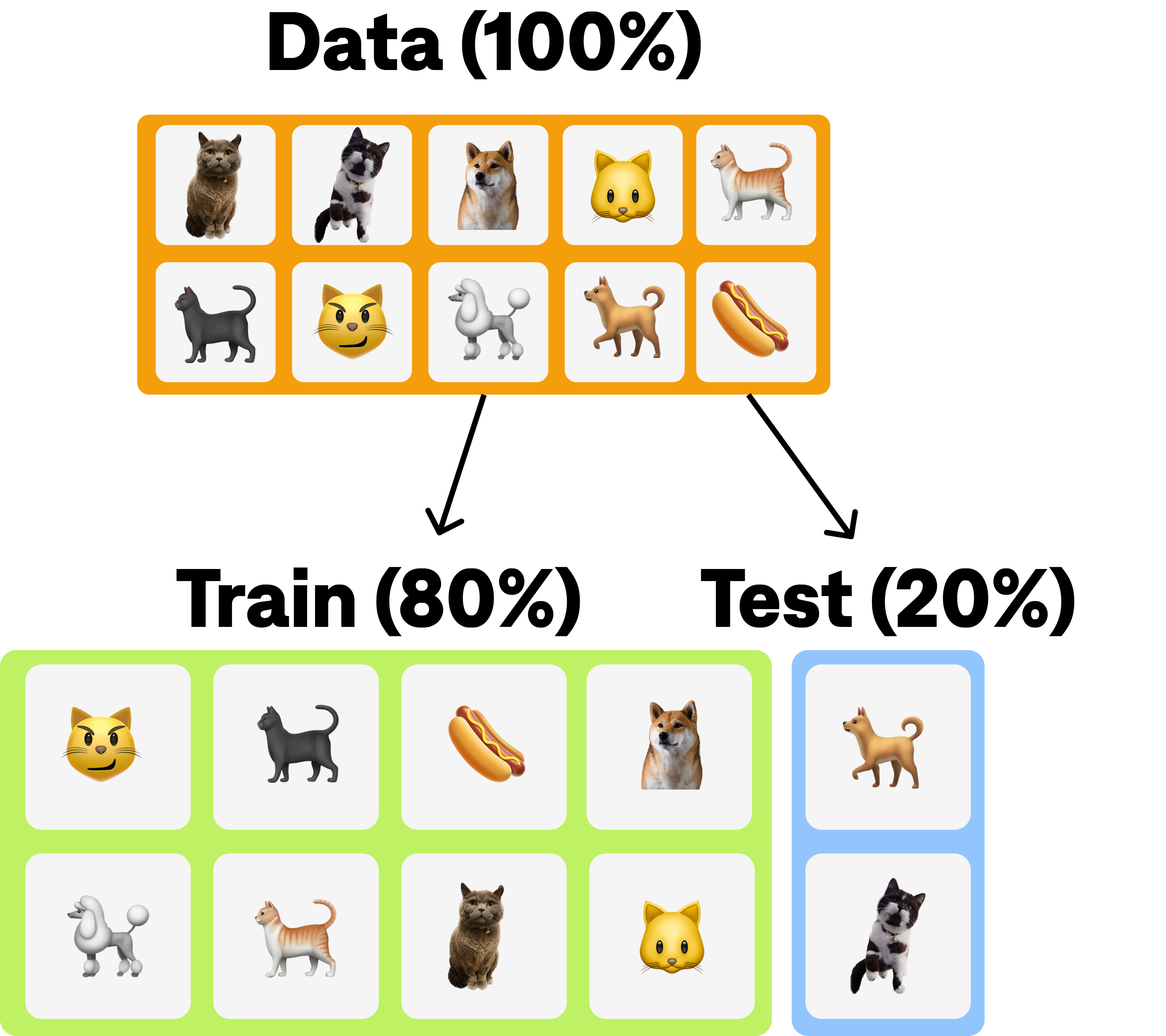
When we want to build a machine learning model, we need to first train it on some data so that it can learn patterns and relationships within that data. However, we also want to know how well our model will perform on new, unseen data. That's where the train/test split comes in.
A train/test split is a way of dividing our data into two parts: a training set and a testing set. We use the training set to train our model, and we use the testing set to evaluate its performance. This allows us to see how well our model is able to generalize and make predictions on new data that it hasn't seen before.
The most common way of doing a train/test split is to randomly divide the data into two sets. By default, PREDICT uses 80% of the data for training and 20% for testing. We also use stratification, so that the train and test set contain approximately the same distribution of classes.
Currently, we don't expose this as a tunable hyperparameter, but will eventually allow users to change it if desired.
Imbalanced Data
Imbalanced data in classification occurs when we have a disproportionate number of examples in one category compared to the others. For example, if we are trying to classify whether a credit card transaction is fraudulent or not, we might find that only a small fraction of transactions are actually fraudulent.
This can create problems for machine learning algorithms because they are often designed to optimize accuracy, which is not necessarily the best metric to use when the data is imbalanced. For example, if we have a dataset with 99% of examples belonging to one class and 1% belonging to another, a model that simply predicts the majority class every time will be 99% accurate, but it won't be very useful in practice.
Infer solves this problem by reweighting the importance of each class. For example, if we have a dataset with 100 images, 90 of them are dogs and 10 are cats, we give a weight of 9 to the cat class and 1 to the dog class. This means that during training, each cat image will contribute 9 times more to the objective than each dog image. This will help the model to focus more on the cat images and improve its accuracy on this underrepresented class.
Default Parameters
We use the default parameters for XGBoost, except the maximum depth is set to 3. We chose this value through experimentation, as it reduces the chance of overfitting, is more computationally efficient, does not dramatically alter the feature importances derived from a model with larger depth.
We currently do not expose the hyperparameters of XGBoost, but plan to do so soon.
We do offer hyperparameter optimisation for PREDICT, which is discussed in the Hyperparameter Optimisation section.
Early Stopping
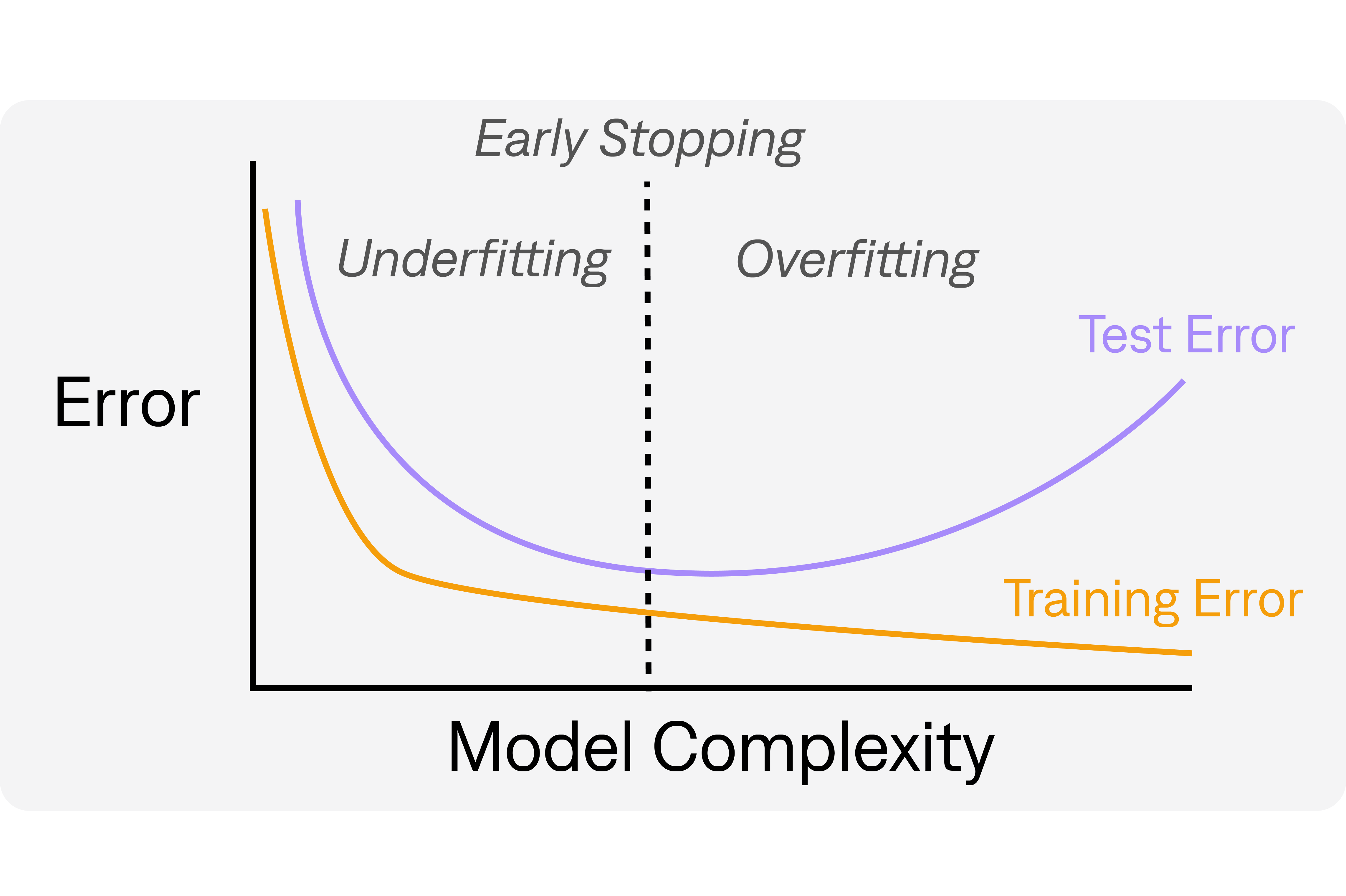
Early stopping is a technique used in machine learning to prevent a model from overfitting the data it has been trained on.
When a model is trained, it learns to fit the patterns in the training data, which may not necessarily generalize well to new, unseen data. Overfitting occurs when the model becomes too complex and starts to fit the noise in the training data as well, leading to poor performance on new data.
Early stopping works by monitoring the model's performance on a validation set (data that the model has not seen during training) during the training process. The validation set is used to estimate the model's performance on new, unseen data. As the model is being trained, its performance on the validation set is evaluated periodically, and if it stops improving, the training is stopped early.
In simpler terms, early stopping is like stopping the model training before it memorizes everything it has seen so far, to prevent it from being too specialized on the training data and perform better on new data.
PREDICT uses an early stopping patience of 20, i.e. if the model has not improved after 20 iterations, it will stop training and use the best model according to the validation set.
Model Evaluation
Model evaluation is the process of assessing the performance of a machine learning model in order to determine how well it is able to make accurate predictions on new, unseen data.
One of the most common methods of model evaluation is to split the available data into a training set and a testing set. The model is then trained on the training set and its performance is measured on the testing set. This approach is known as holdout validation. This is the method we employ at Infer.
There are a range of performance metrics that can be used to evaluate the quality of a machine learning model, including accuracy, precision, recall, mean absolute error, etc.
For PREDICT, the metrics used for evaluation depend on whether you are doing regression (model='reg') or classification (model='clf').
Classification
Metrics
There are several techniques used for evaluating the performance of classification models. Some of the most commonly used techniques include:
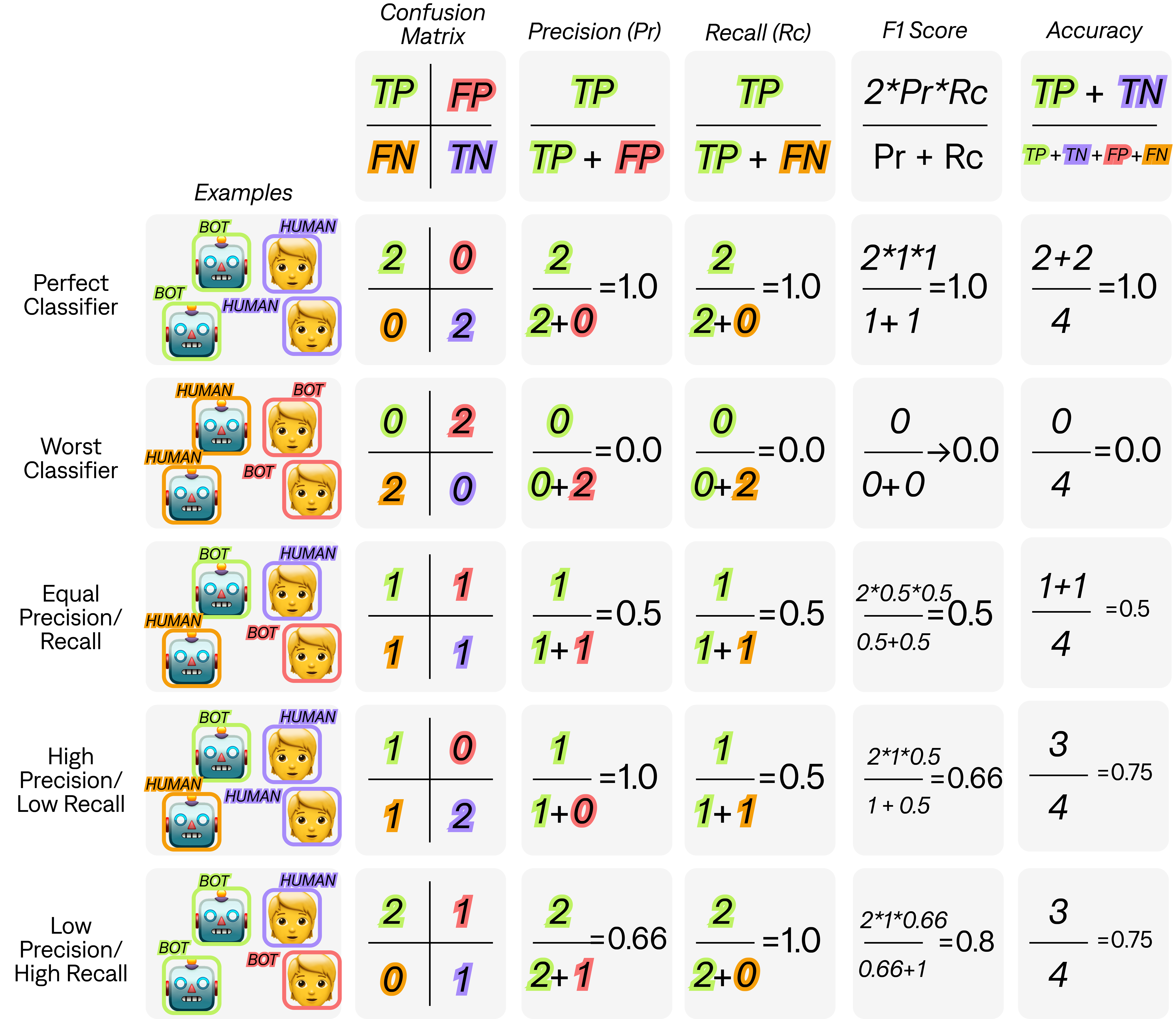
- Accuracy: The accuracy of a classification model is the percentage of correctly classified instances over the total number of instances in the dataset. In other words, it measures the proportion of all correctly predicted values to the total number of values.
- Precision: Precision is the proportion of true positives (TP) among all predicted positives (TP + false positives (FP)). In other words, it measures how often the model correctly identifies positive instances.
- Recall: Recall is the proportion of true positives (TP) among all actual positives (TP + false negatives (FN)). In other words, it measures how often the model correctly identifies actual positive instances.
- F1 score: The F1 score is the harmonic mean of precision and recall. It provides a way to balance the two metrics and is often used as a single metric to evaluate the overall performance of a classification model.
In the below illustration, we show examples of how these metrics are calculated with a bot detection classification model, where BOT represents behaviour from a bot, and HUMAN represents behaviour from a human.
The choice of which metric to optimize for when evaluating a classification model depends on the specific problem at hand and the cost of different types of errors. In general, different metrics prioritize different aspects of the model's performance, and the choice of metric depends on the goals of the model and the domain in which it will be used. Here is a brief overview of when you would want to optimize for each metric:
- Accuracy: Optimizing for accuracy is generally appropriate when the cost of false positives and false negatives is roughly equal. This metric is also appropriate when the classes are balanced, meaning that there are roughly equal numbers of instances in each class.
- Precision: Optimizing for precision is appropriate when the cost of false positives is high. For example, in medical diagnosis, a false positive diagnosis can lead to unnecessary and potentially harmful treatments. In this case, it is important to minimize false positives, even if it comes at the cost of increased false negatives.
- Recall: Optimizing for recall is appropriate when the cost of false negatives is high. For example, in fraud detection, a false negative can result in significant financial loss. In this case, it is important to minimize false negatives, even if it comes at the cost of increased false positives.
- F1 score: The F1 score is a balanced metric that combines both precision and recall. It is useful when the classes are imbalanced, meaning that there are significantly more instances in one class than in the other. In this case, optimizing for accuracy may not be appropriate, as a model that simply predicts the majority class will achieve high accuracy. The F1 score is useful because it takes into account both precision and recall, providing a balanced measure of the model's performance.
The choice of which metric to optimize for depends on the specific problem at hand and the relative cost of different types of errors. It is important to carefully consider the goals of the model and the domain in which it will be used in order to make an informed choice about which metric to optimize for.
Infer calculates all of these metrics automatically, and can be accessed using EXPLAIN.
As explained in Model Training, we automatically reweight the importance of classes during training, so class imbalance does not significantly affect the outcome of the model.
If using our hyperparameter optimisation option, Infer will automatically optimise for F1 score. We plan to allow optimisation of other metrics soon, but find this is the most appropriate metric for many applications.
Regression
Metrics
There are several techniques used for evaluating the performance of regression models. Some of the most commonly used techniques include:
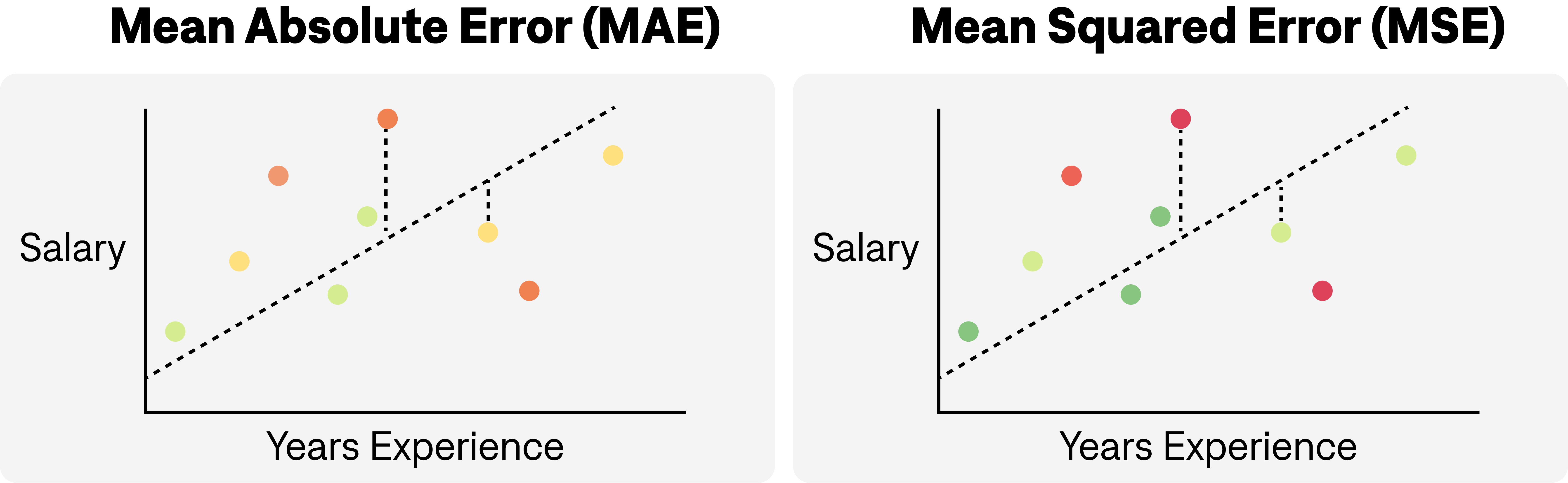
- Mean Absolute Error (MAE): This metric measures the average absolute difference between the predicted and actual values of the dependent variable. It is calculated by taking the absolute value of the difference between the predicted and actual values for each observation, and then taking the average across all observations. Lower values indicate better performance.
- Mean Squared Error (MSE): This metric measures the average squared difference between the predicted and actual values of the dependent variable. It is calculated by squaring the difference between the predicted and actual values for each observation, and then taking the average across all observations. Higher values indicate worse performance.
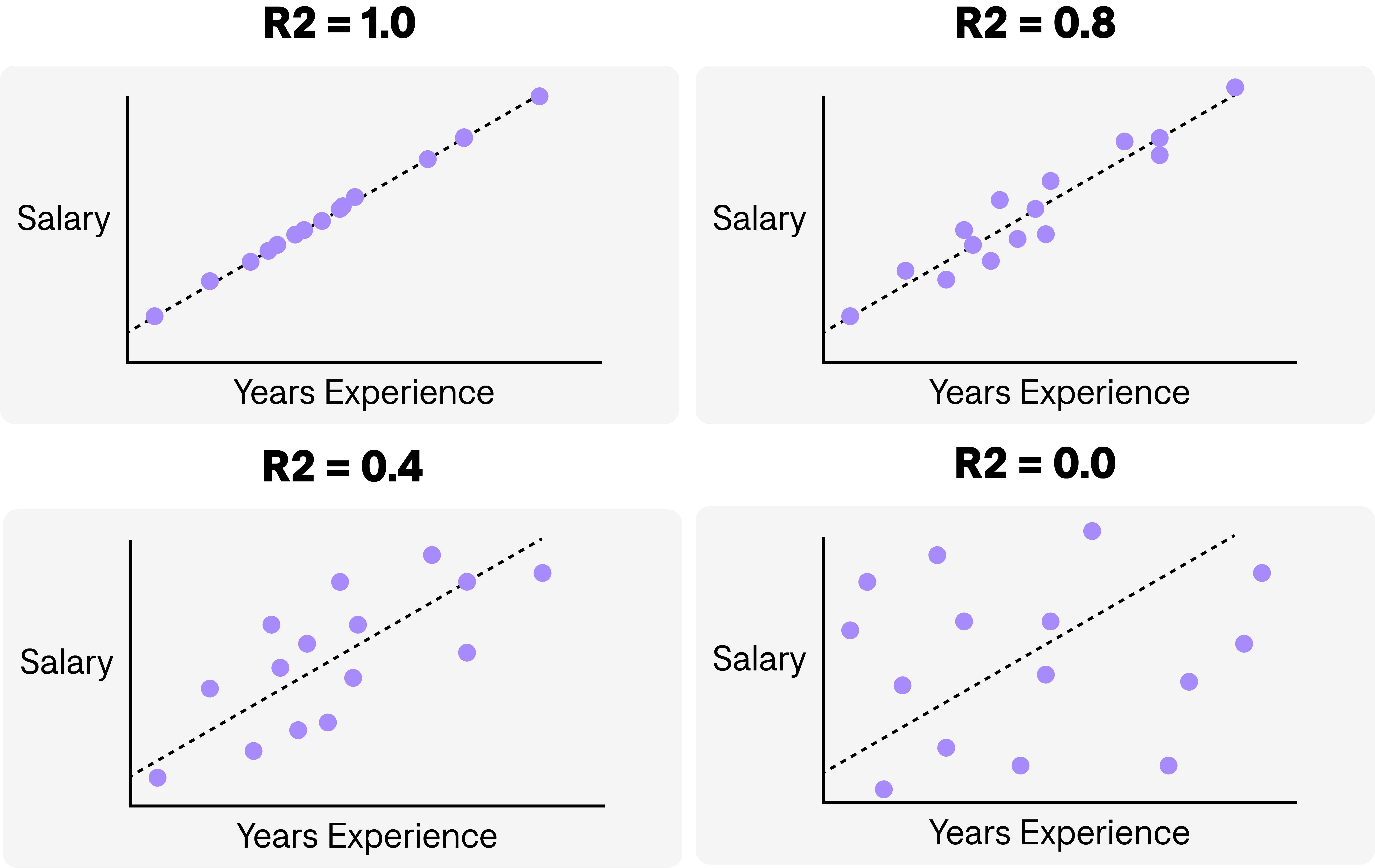
- R-squared (R2): This metric measures the proportion of variance in the dependent variable that is explained by the independent variables in the model. It ranges from 0 to 1, with higher values indicating better performance.
Each metric used in evaluating regression models has its own strengths and weaknesses, and the choice of which metric to optimize for depends on the specific context and goals of the analysis. Here are some reasons why you might want to optimize for each of the commonly used regression evaluation metrics:
- Mean Absolute Error (MAE): This metric is useful when you want to minimize the average difference between the predicted and actual values of the dependent variable. MAE is robust to outliers, since it takes the absolute value of the differences, making it less sensitive to extreme values in the data. Optimizing for MAE may be appropriate when the cost of underestimating and overestimating the dependent variable is similar.
- Mean Squared Error (MSE): This metric is useful when you want to minimize the average squared difference between the predicted and actual values of the dependent variable. MSE penalizes larger errors more heavily than MAE, since the errors are squared. It is commonly used in regression analysis and is often used as a loss function in machine learning algorithms. Optimizing for MSE may be appropriate when the cost of larger errors is significantly higher than the cost of smaller errors.
- R-squared (R2): This metric is useful when you want to explain the proportion of variability in the dependent variable that can be explained by the independent variables in the model. R-squared provides a measure of how well the regression model fits the data, with higher values indicating better fit. It is often used in hypothesis testing and in comparing different models. Optimizing for R-squared may be appropriate when the goal is to understand the underlying relationship between the independent and dependent variables and to identify the most important predictors.
The choice of which metric to optimize for depends on the specific problem at hand and the relative cost of different types of errors. It is important to carefully consider the goals of the model and the domain in which it will be used in order to make an informed choice about which metric to optimize for.
Below, you can see how MSE and MAE differ visually. The main difference is that MSE penalizes larger values more than MAE.
Below we have an illustration of how R2 varies with how well a model explains the variation in the outcome (salary).
Infer calculates all of these metrics automatically, and can be accessed using EXPLAIN.
If using our hyperparameter optimisation option, Infer will automatically optimise for R2. We plan to allow optimisation of other metrics soon, but find this is the most appropriate metric for many applications.
Predictions
Predictions are performed on the entire dataset, which includes the training set, the test set, and missing values.
Predictions using missing values are the ultimate goal - you are predicting the unknown, the future! Select these kinds of future predictions by using WHERE <target> IS NULL AND prediction is NOT NULL.
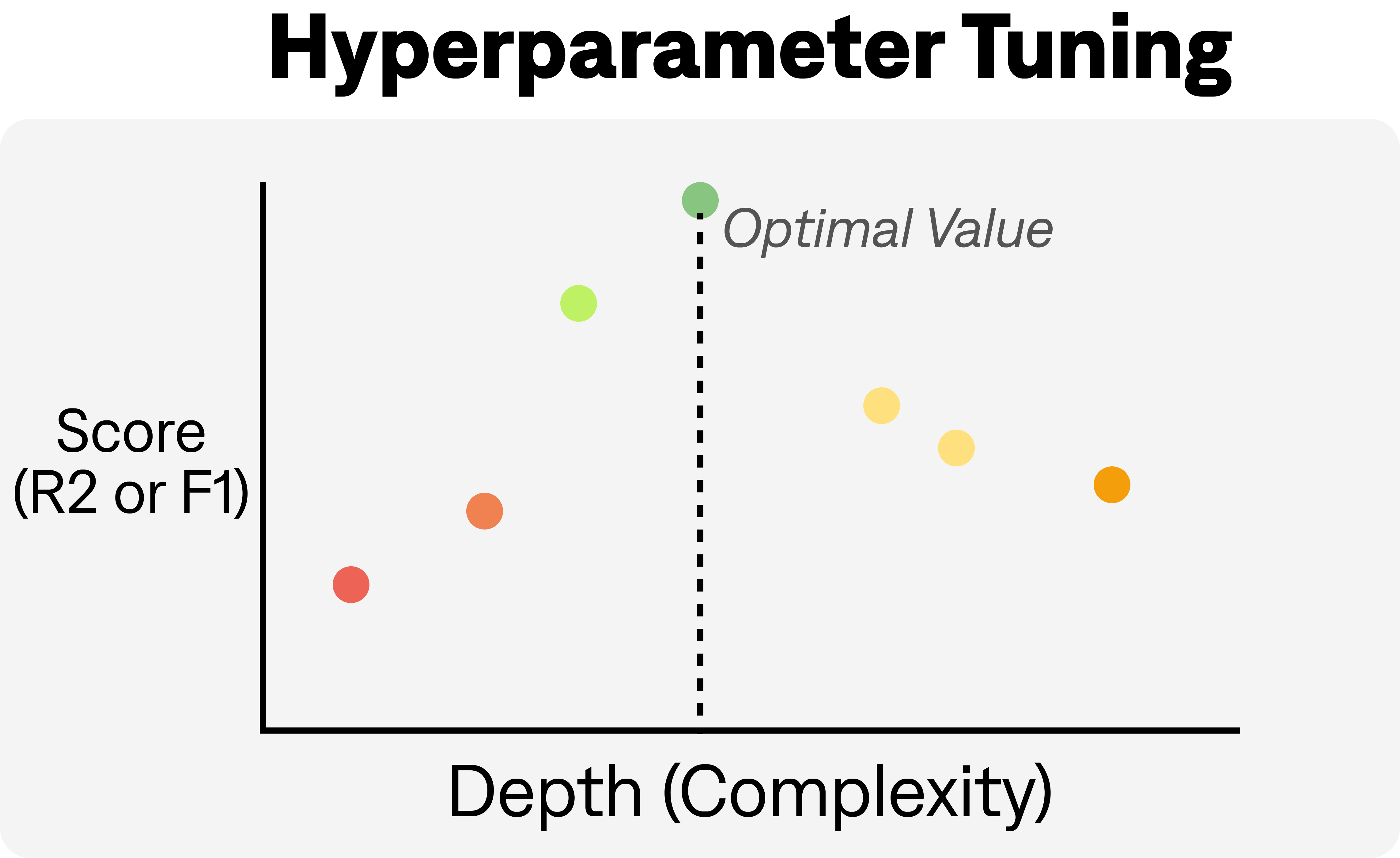
[Optional] Hyperparameter Optimisation (HPO)
Hyperparameter optimization (HPO) is the process of tuning the hyperparameters of a machine learning algorithm in order to maximize its performance on a given task. Hyperparameters are settings of the machine learning algorithm that are set before training, and are not learned from the data.
Hyperparameter optimization involves trying out different combinations of hyperparameters and evaluating the performance of the model on a validation set. This process is done using a search algorithm.
The goal of hyperparameter optimization is to find the hyperparameters that result in the best performance on the test set, while avoiding overfitting to the training set. By optimizing hyperparameters, machine learning models can be trained to achieve better accuracy, generalization, and robustness, and ultimately deliver better results on real-world tasks.
At Infer we use the default search algorithm in Optuna. This algorithm works by creating a population of potential solutions given a search space (all possible combinations of hyperparameters), then uses a combination of genetic algorithms and sorting methods to evolve the population towards the best possible solutions.
The illustration below shows how changing the model complexity (maximum depth) might affect how effective the model is by maximising the F1 score or R2 score.
Use PREDICT(<column>, use_automl=True) to perform HPO on your predictive mode. This will maximize the F1 score for classification (model='clf'), and R2 for regression (model='reg').
Search Space
We currently use 100 trials or 10 minutes of search time (whichever comes first) to find the best possible model with HPO. In the future we will allow users to alter these default settings.
We optimize the following hyperparameters for XGBoost over a wide range of values:
lambda, alpha, subsample, colsample_bytree, max_depth, min_child_weight, eta, gamma, grow_policy.
Model Explainability
Model explainability refers to the ability to understand and interpret the inner workings of machine learning models. It involves identifying and understanding how a model makes decisions or predictions based on the data it has been trained on.
Model explanations can be a powerful tool for understanding the drivers of a particular outcome and finding insights that may not be immediately apparent from the data alone. Here are a few ways that you can use model explanations for this purpose:
- Identify important features: One of the most basic uses of model explanations is to identify which features or variables have the strongest relationship with the outcome you are interested in. This can help you to focus your analysis on the most important drivers and identify potential areas for further investigation.
- Understand nonlinear relationships: In many cases, the relationship between the outcome and the predictors may be nonlinear, meaning that the relationship changes depending on the value of the predictor. Model explanations can help you to understand these nonlinear relationships by showing how the predicted outcome changes as the value of the predictor changes.
- Identify outliers: Model explanations can also help you to identify outliers or unusual data points that may be driving the prediction. By examining the explanations for these outliers, you may be able to uncover insights that were not apparent from the data alone.
In general, model explanations can help you to understand the drivers of a particular outcome by providing a detailed view of how the model is making its predictions. By using these explanations to focus your analysis and uncover insights, you can gain a deeper understanding of the problem you are trying to solve and make more informed decisions.
EXPLAIN uses two main methods to explain what your predictive model has learned: feature importance, and SHAP.
Global vs Local Explanation
In the context of machine learning models, global and local model explanations refer to two different ways of understanding how a model is making its predictions.
- Global model explanations: These are explanations that describe how a model makes predictions across an entire dataset or population. Global explanations help us to understand which features are most important for the model overall, and how those features interact with each other to produce predictions. Feature Importance and SHAP are two commonly used techniques for generating global model explanations.
- Local model explanations: These are explanations that describe how a model makes predictions for a specific instance or observation within a dataset. Local explanations help us to understand why a model is making a particular prediction for a particular instance, and can be useful for identifying biases or errors in the model. SHAP is a commonly used technique for generating local model explanations.
Feature Importance
Feature importance is a technique used in machine learning to identify the most important variables or features that contribute to the accuracy or predictive power of a model. In other words, it helps to determine which features have the greatest impact on the outcome being predicted.
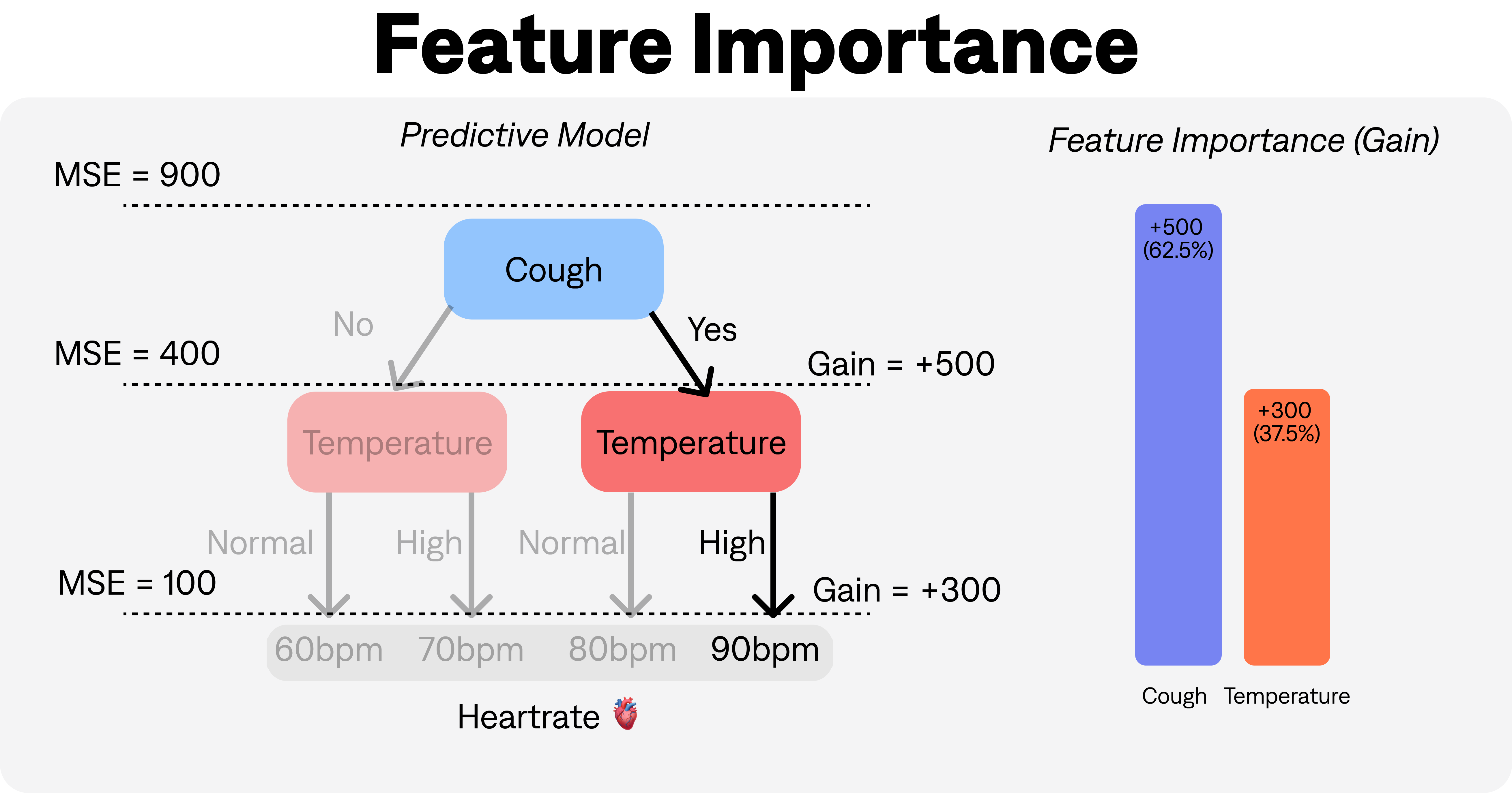
EXPLAIN calculates feature importance based on how much each feature contributes to reducing the impurity of the decision trees used in the gradient boosting process (the algorithm used by PREDICT).
In particular, we use the gain version of feature importance. This represents the relative contribution of each feature to the model calculated by the sum of the gain over all splits that use the feature. The gain is calculated as the improvement in the objective function (e.g., log loss or mean squared error) brought by that feature.
Large gains means that feature contributed a lot to accurately predicting the outcome, vice versa for small gains.
When using EXPLAIN, we return feature importance for binary classification and regression models. For multi-class classification, we use aggregated SHAP.
Below is an illustration of how the feature importance is calculated for a decision tree model predicting the resting heartrate of a person given some information about whether they have a cough or a temperature.
SHAP
SHAP (SHapley Additive exPlanations) is a technique for generating both global and local model explanations. SHAP is based on the concept of game theory, and calculates the contribution of each feature to a prediction using a method called Shapley values. SHAP values can be used to generate both global feature importance rankings and local explanations for individual predictions. The advantage of using SHAP over other methods is that it provides an intuitive way to understand the contribution of each feature to a prediction, and can be used with a wide range of machine learning models.
To learn more about SHAP, see here.
For multi-class classification problems, Infer uses SHAP to calculate local explanations, then aggregate them to produce feature importances. This allows us to assign feature importances to each class, rather than just an overall score to each feature. You can think of SHAP as a more complicated version of Feature Importance, but overall operates in a similar way - measuring the 'gain' due to contributions of different columns and data points.
Auto-viz
Automatic visualization of results from SQL queries using Infer can significantly accelerate time-to-insight. With the increased complexity of adding machine-learning methods to your SQL, and the handling of the extra data generated by that process, it can be challenging to quickly identify patterns or trends without visual aids.
Because Infer knows which commands you are using, we can automatically build charts and reports that are the most informative based on what you are trying to do.
Visualisations are based on the last Infer command you used in your query. Infer can only plot information that is returned by the user, so if write a nested SELECT statement and remove or alter variables, omitted and derived variables will not be visualised.
As such we generally recommend returning all data from PREDICT or EXPLAIN instead of subselecting.